Usage
Several ways are possible to use the application
- Direct from the web: Just click on "Start TinT". That starts the graphical application direct from the browser local on your computer in a separate window. For further help see on the menu line in the application "Help -> Usage".
-
Manually on your computer: First download the
application here and then execute in
a terminal
java [-Xmx512m] -jar tint.jar
the parameter -Xmx is not neccessary, but sets the maximum memory consumed by Java. Here is is set to 512MB. If the application hangs, it could be neccessary to encrease the value (like -Xmx1024m). - Command line version: For details see here
Remarks
Reading data (esp the data from the servers called "Remote RM data") may take minutes to finish, depending on the internet connection. To avoid reading again over internet there is an option in the menu called "Download RM data". Here you may select files and store them locally on your computer. This may improve your evaluation time.
Error Messages
Error messages are written (added) into a file called tint.log in the folder $HOME/.bioinf (on unix machines) or the appropriate folder .bioinf in your user's directory in Windows. In case of failures it is a good idea to send the tint.log file along with a failure message.
File Formats
RepeatMasker
   SW  perc perc perc  query      position in query           matching       repeat              position in  repeat
score  div. del. ins.  sequence    begin     end    (left)    repeat         class/family         begin  end (left)   ID

  221  28.7  0.6  8.3  scaffold_0     167     322   (75329) +  CT-rich        Low_complexity           1  144    (0)      1
  255  29.0  2.2  6.1  scaffold_0     306     485   (75166) +  C-rich         Low_complexity           4  176    (0)      2
  223  21.3  0.0  4.1  scaffold_0    2073    2121   (73530) +  G-rich         Low_complexity           2   48    (0)      3
  412  24.8  9.6  1.9  scaffold_0    2935    3090   (72561) +  MLT1A          LTR/MaLR                 1  168  (206)      4
  238  19.2  3.9  0.0  scaffold_0    9145    9196   (66455) +  L1MC           LINE/L1               3675 3728 (2418)      5
  272  19.4  0.0 14.3  scaffold_0    9205    9288   (66363) +  tRNA-Lys-AAG   tRNA                     1   72    (4)      6
  850   7.9  0.0  0.8  scaffold_0    9289    9415   (66236) +  SINEC_Fc2      SINE/Lys                90  215   (10)      7
 2318  19.7  5.0  7.0  scaffold_0    9422    9830   (65821) +  L1MC           LINE/L1               3732 4163 (1983)      5
  912  21.7  6.5  3.7  scaffold_0    9831   10045   (65606) +  SINEC_Fc2      SINE/Lys                 1  221    (4)      8
 2318  19.7  5.0  7.0  scaffold_0   10046   10291   (65360) +  L1MC           LINE/L1               4164 4374 (1772)      5
  749  18.5 13.7  4.9  scaffold_0   11098   11302   (64349) +  SINEC_Fc2      SINE/Lys                 3  225    (0)      9
  774  30.5 17.7  2.7  scaffold_0   12157   12895   (62756) +  L1MC3          LINE/L1               6618 7467  (318)     10
  318  31.8  4.5  3.0  scaffold_0   16128   16260   (59391) +  MIR            SINE/MIR                53  187   (75)     11
Header lines are discarded while loading and it is essential that each data line include the ID number! Perc: xxxx, div: xxx, del: xxxx, ins: xxx, etc. for all abbreviations.
TinT
AluJb[SINE/Alu] 3       19      0       1       1       0       1       0       25279   1       274.5
AluJo[SINE/Alu] 2       22      0       0       0       1       0       0       27779   1       263.3
AluSc[SINE/Alu] 7       21      0       3       0       1       7       0       9508    1       296.5
AluSg[SINE/Alu] 8       15      3       0       0       1       13      0       16935   1       312.6
AluSp[SINE/Alu] 8       13      0       1       0       2       11      0       10366   1       311.3
AluSq[SINE/Alu] 6       23      2       1       1       1       7       0       17939   1       306.1
AluSx[SINE/Alu] 37      88      1       3       1       5       14      1       63713   1       309.5
AluY[SINE/Alu]  17      43      8       5       3       10      43      2       27919   1       309.0
In the first column there are the names of transpositions together with the listed families/classes. The last 3 columns contain (1) the count, (2) a time-scale factor (reserved) and (3) an average size (length) of the elements analyzed elements. The other columns contain the count of transpositions t(i) inside t(j) where i denotes the row and j the column.
Configuration File
[SINE Check]
qlen=20
rext=50
rextover=18
rover=35
strongcond=true

[CR1 Check]
qlen=20
rext=50
rextover=24
rover=12
gap=50

[Family Colors]
LINE/CR1=128,128,128
LINE/I=128,128,128
LINE/Jockey=128,128,128
LINE/LOA=128,128,128
LINE/R1=128,128,128
LINE/R2=128,128,128
LINE/telomeric=128,128,128
LTR/Copia=128,128,128
LTR/Gypsy=128,128,128
LTR/Pao=128,128,128
SINE/Alu=128,128,128

[Trans Colors]
AluJb=0,128,128
AluSc=255,128,128
DMCR1A=191,128,128
MDG1=255,128,128

[Merging]
ALU=Alu1,Alu2,LINE/CL
XYZ=SINE,SINE/CL
SINE/CR1 Check
- qlen: (Minimum query length) The minimum length of transpositions to be recognized.
- rext: (Minimum repeat extension) The valid distance of tp and tn.
-
If rext fails:
rextover, rover: (Minimum repeat extension overlay), (Maximum repeat overlay) It is the valid distance and overlay of tp and tn. - stongcond: (Strong condition) Select possible insertions more or less "precisely". Strong means: id, orientation and name of tp and tn are equal. Otherwise only name and family/class of tp and tn are checked.
Merging
Using Graphical TinT
After starting the application you will find a pull down menu at the top of the application. The option File allows you to load and store information
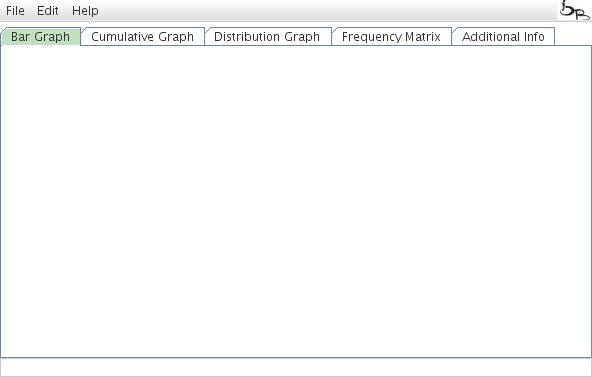
Figure 1: Input mask after starting the TinT application.
Load RepeatMasker Files
The initial step is to load Repeat Masker data. There are three options
- use the ready to use Repeat Masker files that we have prepared for reference species (e.g., from Churakov et al. 2010, Homo_Alu.out)
- RepeatMasker files can be uploaded from a URL
- you can upload local RepeatMasker files.
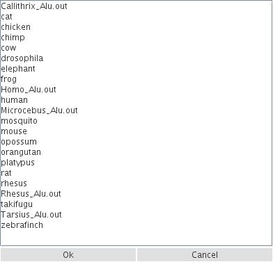
Figure 2: Example for loading predefined RepeatMasker data from representative species or from current TinT publications.
After loading RepeatMasker data from a selected species (this can take a while, the progress is indicated on the bottom line) a table of element families and subfamilies will appear (entitled: Select Elements). Select the group of elements to calculate their TinTs (please note that the selected data are reloaded and they replace the original data input to keep the memory usage of the local computer as low as possible).
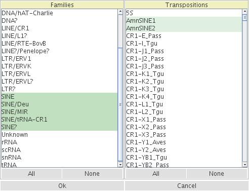
Figure 3: Mask to select specific elements for TinT.
Calculate values and generate graphs
After selecting your elements of interest, a Bar Graph of retroposon activity appears. If desired, the colors for specific bars can be adopted by clicking on the ovals and selecting the color from the color spectrum (alternatively, colors can be changed via the Edit menu. It is also possible to set retroposon colors corresponding to family affiliations.
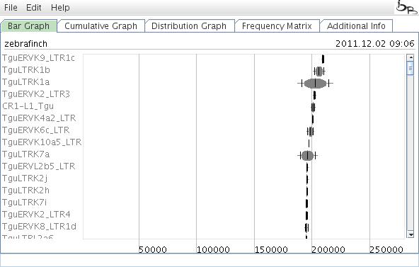
Figure 4: Results of a TinT analysis displayed in the Bar Graph.
At this stage you can save the frequency file (click: File and Save Frequency File) for reuse in a later run without having to reload the full data again.
Changing the parameters of TinT
Select Edit and Set Parameters from the pull down menu. Select the retroposon type (default: SINE or CR1). The Select Element table appears with the preselected elements. Parameters can be changes individually (see Churakov et al. 2010, Matzke et al. 2012). The TinTs will be calculated applying the changed parameters after reloading the data.
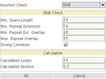
Figure 5: Standard parameters for a TinT run. For explanation see Churakov et al. 2010.
Merge Transpositions
Select Edit and Merge Transpositions from the pull down menu. Add a new group name and select the Free Elements that should be merged. Move them with the "<" option to the Merged Elements field. Select these elements in the Merged Elements field. Print a name for the merged elements and press Add. The new graph with the merged elements will appear.
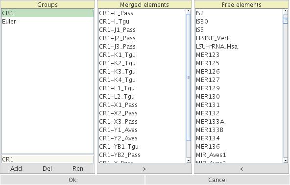
Figure 6: Merging elements in the Merged Elements field from the complete set in the Free Elements field. The new name C1 is designed for the merged elements.
Alternative displays of the TinT results
You can choose the Cumulative Graph to see the cumulative probability of retrotransposon activity. This graph presents periods of high/low retroposon activity and/or changes in the population size over time. Colors of specific element activities can be adopted corresponding to the Bar Graph option as described above. Note that the elements with a large range of activity are placed at the bottom of the graph. Elements with low activity profiles are placed at the top. Move the mouse while pressing the ctrl key will zoom the corresponding region. Pressing the R key will reset to the original size. Clicking with the right mouse bottom in a part of the graph will place the name of the corresponding active element. An additional click will remove the name.
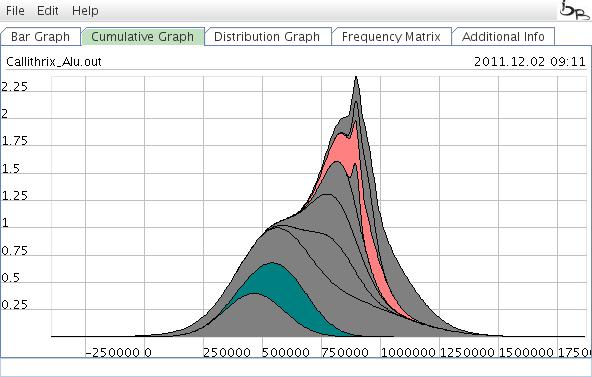
Figure 7: Cumulative Graph representing the accumulated retrotransposon activity probability. It is possible to zoom in on the curve to visualize specific parts of the graph.
The Distribution Graph
The Distribution Graph shows individual curves of retrotransposon activity.
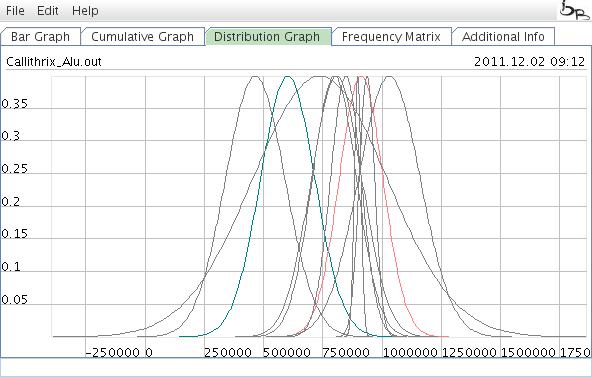
Figure 8: Distribution Graph showing the probabilities of individual element activities .
This graph displays the distribution of the calcualted T(i) values. For the actions inside this graph, see the cumulative graph. Just the "display names" option is not available.
Frequency Matrix
The Frequency Matrix presents the calculated number of nested elements, the total count of elements, the average size of elements, and the T(i) values (a specific value of the TinT algorithm; see Churakov et al. 2010).
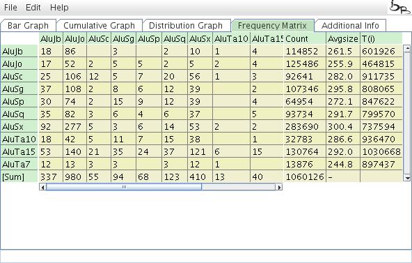
Figure 9: Frequency Matrix of TinT.
Additional information
The Additional Info field displays the tranpositions that are not considered in the TinT calculation, either because they are too old, too young, or represent just a minor fraction of the total elements.
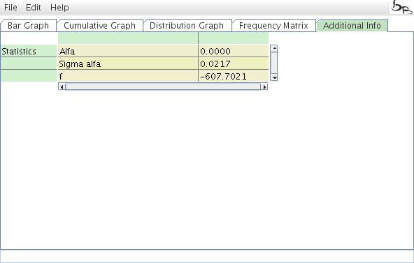
Figure 10: Additional Info table.
Speed up and caching
There is an additional optional feature enabled, which caches names of families and transpositions read from RepeatMasker files in a special file entitled: .bioinf/tint.cache. This helps to speed up the loading of files. If a file is not changed and already read, the names will be saved here, so they can be (re)read instead of having to load the RepeatMasker file twice. Removing the cache file initializes TinT on the next start.